The Central Limit Theorem - Visualized
For this week, I'm finally sharing the code I wrote to produce my visualization demonstrating the Central Limit Theorem! But before we get to the code, I wanted to discuss the impact of this visualization and how it can be interpreted.
What is the Central Limit Theorem?
This is a very brief background & example of the Central Limit Theorem and is not intended to be comprehensive.
The Central Limit Theorem (CLT) establishes that the summation of independent, random variables. The resultant distribution of their normalized sums takes on a normal shape even if the original random variables were not normally distributed themselves.
If you’re not familiar with statistics, that sentence may make absolutely no sense. In that case, think of it this way: say you want to estimate the average height of a given adult (human) population. It would be nearly impossible to measure everyone’s height, so you instead take sample of 30 people and calculate their average height. You then want to generalize and claim that the average height of these 30 people represents the average height of the entire population.
Are we sure this claim can be made? If we were to sample another 30 people and calculate their average height, would we get the exact same answer? While it might be close, we almost certainly would not get the "same" answer, which indicates that there is some amount of sampling bias (changes in the variable of interest due to randomness in our sample).
So where does the CLT come into play? The theorem argues that if we were to repeat the sampling process many times, and then take the average height of each of those samples, those averages would deliver a result similar to a normal distribution. This distribution of averages is called the sampling distribution of the mean (a sampling distribution is just a distribution made up of statistics performed on many samples from the same population) and can be used to reliably estimate the true average height of our population! The best part of the CLT is that even if the population of heights is not normally distributed, the sampling distribution of the mean will be. The upshot here is that the mean of sampled means will be a reliable estimator of the population mean regardless of the shape of the population distribution.
However, we typically cannot sample 30 random people hundreds of times to accurately estimate the average height of the population, so we often rely on the CLT to argue that our single sample should be good enough.
Interpreting the Figure
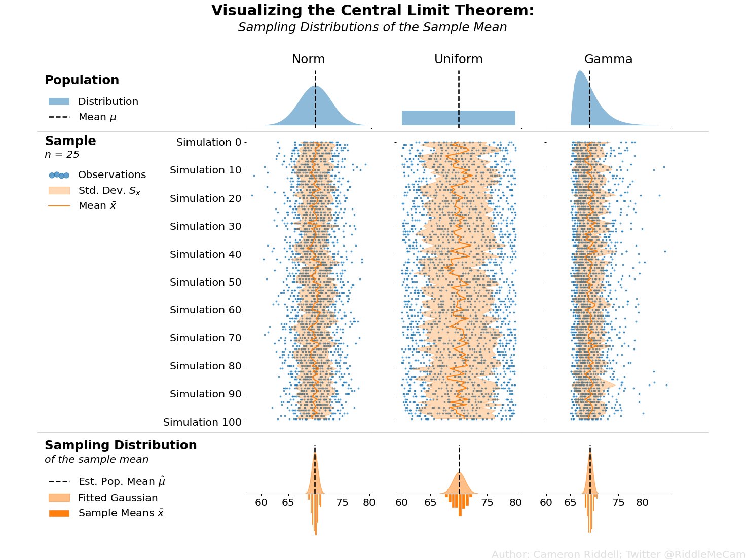
Applied to the above figure, you can think of the population of heights as the first row of plots. If we simulate samples from those populations (blue points in the second row of plots) and overlay the means of each of those samples (dark orange line), you can clearly see the sampling variability of the mean—the amount the dark orange zigs and zags from sample to sample. Then, in the final row of the image, we plot the sampling distribution—essentially a histogram of all of those means we calculated in the second row of plots. The CLT argues that the final row of plots will always approach a normal shape even if the population (first row of plots) is not normally distributed.
Whew! that’s enough statistics talk, let’s get to the actual code!
Creating The Visualization
How would we go about creating the above visualization? I’ll walk you through the steps and code I wrote to make it, highlighting some of the important matplotlib concepts you’ll need to understand to produce high quality visualizations.
I want to preface that I’ll import each specific function I use in each cell of this notebook to keep each section clean and so you can readily map the function back to its import.
Firstly, I set some defaults:
Bump up the font size
Force the figure to have a white background
from matplotlib.pyplot import rc, rcdefaults
from IPython.display import display

rcdefaults()
rc('figure', facecolor='white')
rc('font', size=16)
Figure Layout & Distribution Set Up
With the plotting defaults out of the way, lets set up our populations and create a layout for the visualization. First, I'll create the distributions in scipy. From there, I'll set up my grid. I should note that the gridspec_kw are determined post-hoc (after I finished the final version of the figure) to ensure the layout had no overlapping text and everything was spaced correctly.
Note that you do not need to take this manual approach—relying on matplotlib–to clean up your layout, but it is extremely easy with matplotlibs tight layout and constrained layout. I manually specified my layout to ensure my plot is 100% reproducible without any further tweaks.
By establishing my population distributions first, I can easily add more distributions later without needing to change my plotting code since I generate len(populations) number of columns in my subplots grid.
Additionally, I can readily zip my distribution together with the first row of Axes to create plots on just the top row!
from numpy import linspace
from scipy.stats import norm, uniform, gamma
from matplotlib.pyplot import subplots


## All populations should have central tendency ~70,
#  keeps things comparable across distributions
populations = [
    norm(loc=70, scale=3), uniform(60, 20), gamma(1.99, loc=65, scale=2)
]

fig, axes = subplots(
    3, len(populations), figsize=(20, 16),
    sharex=True, sharey='row',
    gridspec_kw={
        'height_ratios': [1, 5, 1], 'hspace': 0, 'wspace': .1,
        'bottom': .08, 'right': .9, 'left': .3, 'top': .9
    },
    dpi=104
)

for pop, ax in zip(populations, axes[0]):
    xs = linspace(*pop.ppf([.001, .999]), 4_000)
    ax.fill_between(xs, pop.pdf(xs), alpha=.5, label='Distribution')
    ax.axvline(
        pop.mean(), 0, .95, ls='dashed', color='k', lw=2, label=r'Mean $\mu$'
    )
    ax.set_title(pop.dist.name.title(), fontsize='large')

    ax.xaxis.set_tick_params(length=0)
    ax.yaxis.set_tick_params(labelleft=False, length=0)
    ax.margins(y=0)

display(fig)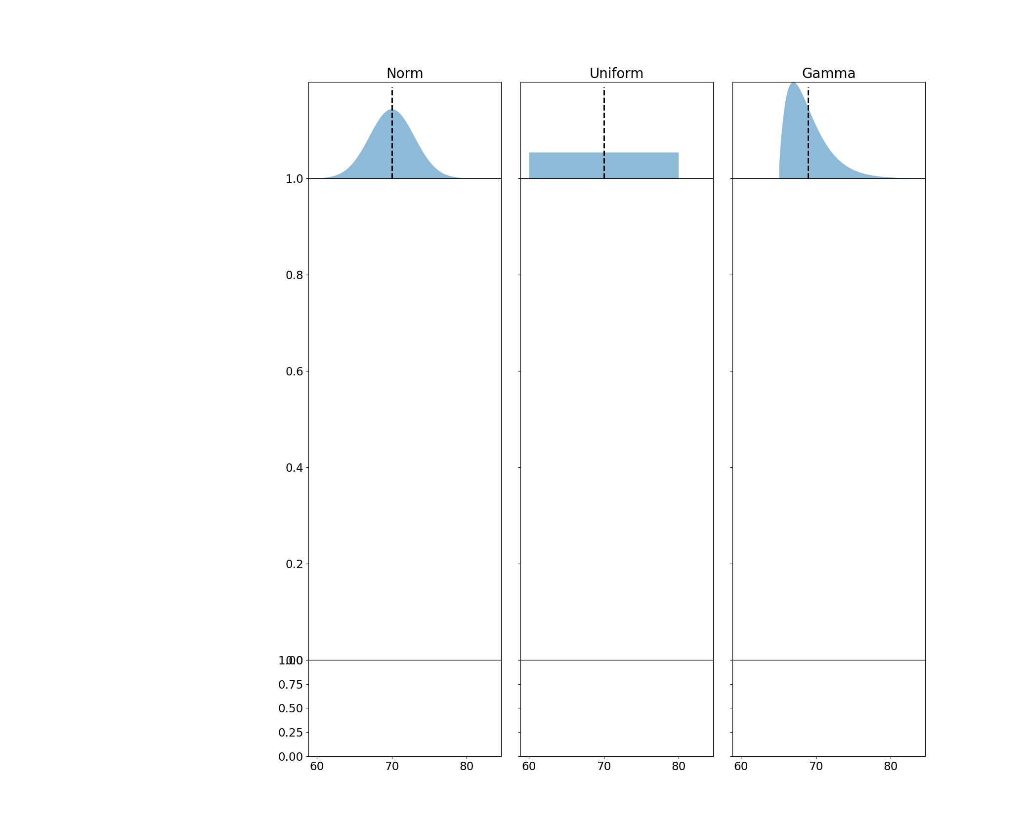
Running & Displaying the Simulation
I then set up my samples from each population distribution. Each sample has a pre-specified size and is re-drawn many times to capture the sampling variability. I use NumPy methods as often as possible to ensure my code runs quickly, and then zip those samples together with the second row of plots to perform the actual plotting. There are also a few other NumPy tricks I use to ensure that my arrays align with each other when performing plotting.
from numpy.random import default_rng
from numpy import arange, broadcast_to

rng = default_rng(0)

n_samples, sample_size = 100, 25
samples = [
    p.rvs(size=(n_samples, sample_size), random_state=rng)
    for p in populations
]

ys = arange(n_samples)
scatter_ys = broadcast_to(ys[:, None], (n_samples, sample_size))
rng = default_rng(0)

for s, samp_ax in zip(samples, axes[1, :]):
    smean, sdev = s.mean(axis=1), s.std(axis=1)

    samp_ax.scatter(
        s, y=scatter_ys, s=4, c='tab:blue', alpha=.7, label='Observations'
    )
    samp_ax.fill_betweenx(
        ys, x1=smean - sdev, x2=smean + sdev, color='tab:orange',
        alpha=.3, label='Std. Dev. $S_x$'
    )
    samp_ax.plot(smean, ys, color='tab:orange', label=r'Mean $\bar{x}$')
    samp_ax.xaxis.set_tick_params(length=0)

display(fig)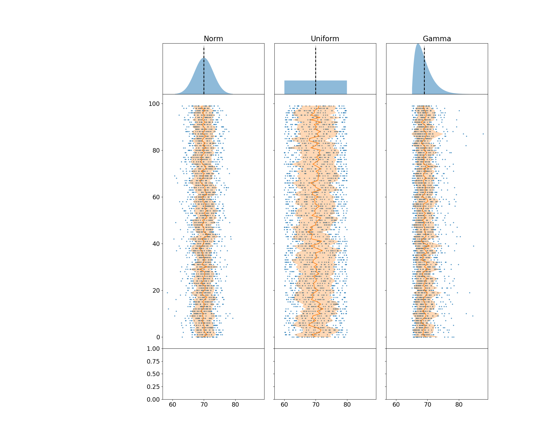
Creating the Sampling Distributions
In the final row of my plot, I create a histogram with a fitted gaussian on the bottom. This is intended to directly map observed values to their smoothed counterpart. I plot the mean of the sampling distribution as a vertical black bar that represents the estimated population average.
for s, mean_ax in zip(samples, axes[2, :]):
    smean, sdev = s.mean(axis=1), s.std(axis=1)

    mean_ax.axvline(
        smean.mean(), ymin=.5, ymax=.9, c='k', ls='dashed',
        lw=2, label=r'Est. Pop. Mean $\hat{\mu}$'
    )

    norm_density = norm(*norm.fit(smean))
    xs = linspace(*norm_density.ppf([.001, .999]), 4000)
    mean_ax.fill_between(
        xs, -norm_density.pdf(xs), label='Fitted Gaussian',
        alpha=.5, color='tab:orange'
    )
    mean_ax.hist(
        smean, bins='auto', label=r'Sample Means $\bar{x}$',
        density=True,  color='tab:orange', ec='white'
    )
    mean_ax.yaxis.set_visible(False)
    mean_ax.spines['bottom'].set_position('zero')

display(fig)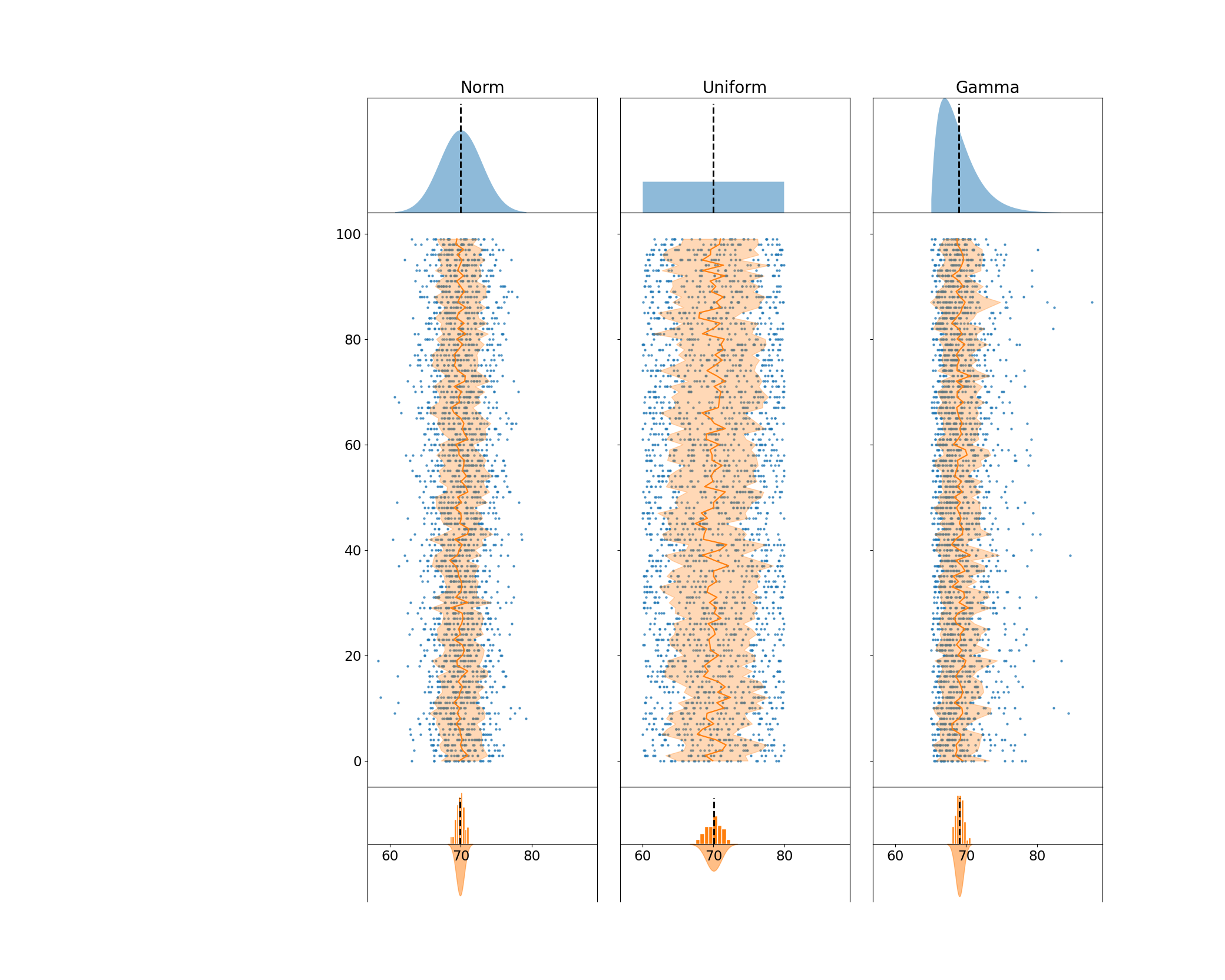
Cleaning Aesthetics
All we have left to do now is a little cleanup. First, I force major ticks to appear on every ten units of the y-axis on the second row of plots. These plots all share a y-axis, so I only need to make the change on one of them. Since the figure is designed to be read from top to bottom, I invert the y-axis so that it increases as the readers' eyes move downwards. I also set the y label and rotate it to ensure its orientation is in line with the downwards count.
Next, I tidy the bottom row of Axes; since all plots share an x-axis, I can uniformly set the x-axis on all of the plots and reduce their margins and center the expected population mean. I also add some extra padding on the y-margin of these plots so the fitted distribution/histograms don’t bump up against their Axes limits.
from matplotlib.ticker import MultipleLocator

## Set custom ticks and limits to the Simulation & Sampling Dist. Axes
# The y-axes are shared across rows of the figure,
# so we only need to invert 1 y-axis out of the row of sample Axes
samp_ax = axes[1, 0]
samp_ax.yaxis.set_major_locator(MultipleLocator(10))
samp_ax.yaxis.set_major_formatter('Simulation {x:.0f}')
samp_ax.invert_yaxis()
# samp_ax.set_ylabel('Simulation', size='large', rotation=-90, va='top')

# Manually set the xlimits, they're shared across all Axes
#   the population means hover ~70, so we drop that xtick for visibility
mean_ax = axes[2, 0]
mean_ax.set(xlim=(60, 80), xticks=[60, 65, 75, 80])
mean_ax.invert_yaxis() # flip the histgram and KDE, so the KDE is on top
mean_ax.margins(y=0.1)

display(fig)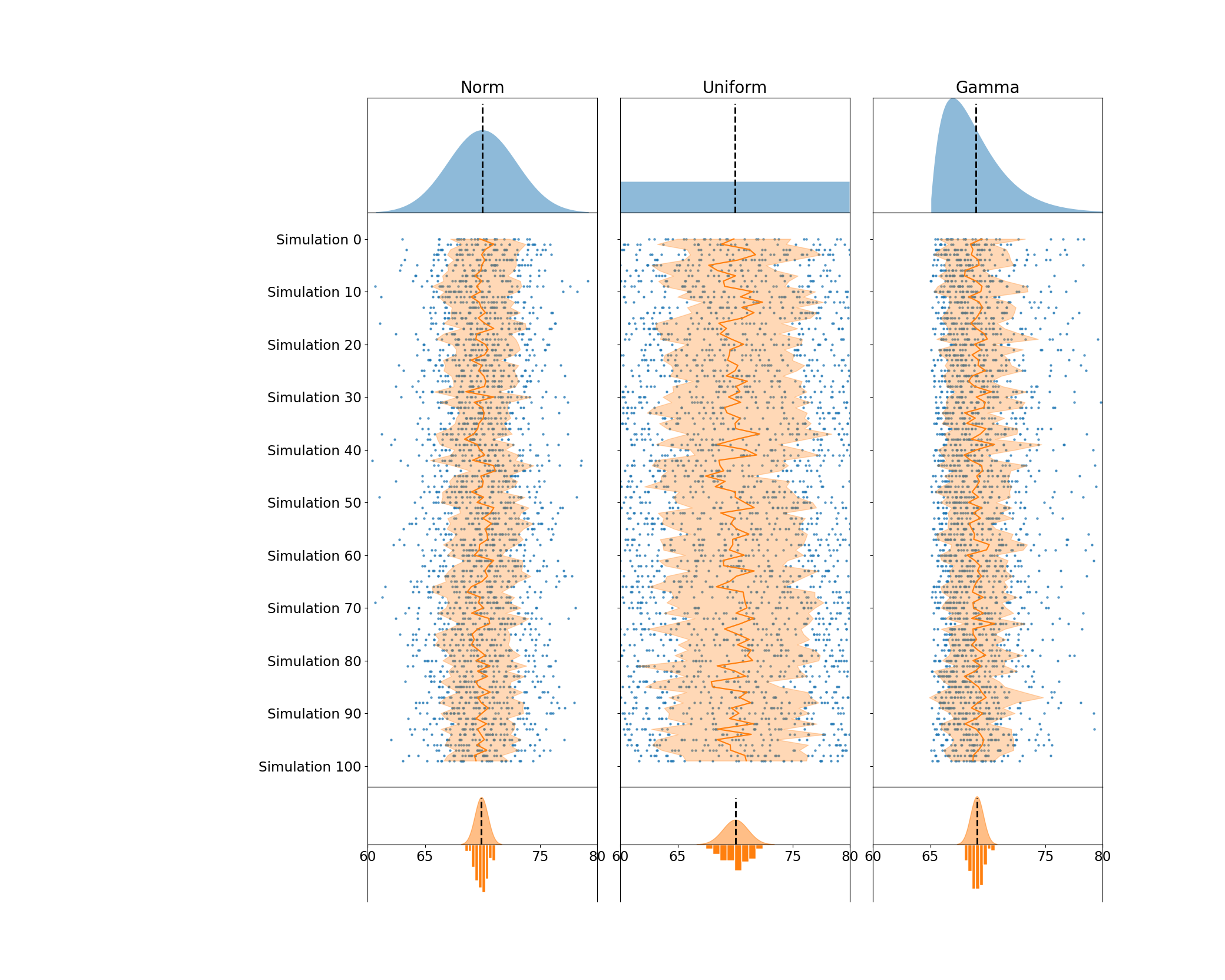
Adding Text Annotations & Legends
Now I want to add some descriptive legends I'll use to annotate my figure. To do this, I rely on matplotlibs internal Legend generation from the Axes.legend. However, I want to add custom titles and subtitles to these plots. Do to this, I use a little trick of decomposing the legends via their .get_children() method and pack on my own TextArea to have explicit control over multiple fonts, the title spacing, and alignment with the Legend.
from matplotlib.transforms import blended_transform_factory
from matplotlib.offsetbox import VPacker, TextArea, AnchoredOffsetbox

## Create left-aligned titles for each row
axes_titles = [
    ('Population', ''),
    ('Samples', f'n = {sample_size}'),
    ('Sampling Distribution', 'of the sample mean')
]
for (title, subtitle), ax in zip(axes_titles, axes[:, 0], strict=True):
    titlebox = [
        TextArea(title, textprops={'size': 'large', 'weight': 'semibold'})
    ]
    if subtitle:
        titlebox.append(TextArea(subtitle, textprops={'style': 'italic'}))
    title_packer = VPacker(pad=0, sep=5, children=titlebox)

    legend = fig.legend(
        *ax.get_legend_handles_labels(), markerscale=4, scatterpoints=4
    )
    legend.remove()

    # Legends are composed of two children: VPacker & FancyBboxPatch
    #   We can extract the VPacker and add it to our own for a very custom title
    legend_body, _ = legend.get_children()
    transform = blended_transform_factory(fig.transFigure, ax.transAxes)
    fig.add_artist(
        AnchoredOffsetbox(
            loc='upper left',
            child=VPacker(
                align='left', pad=10, sep=10,
                children=[title_packer, legend_body]
            ),
            bbox_to_anchor=(0.05, 1), bbox_transform=transform,
            borderpad=0, frameon=False
        )
    )

display(fig)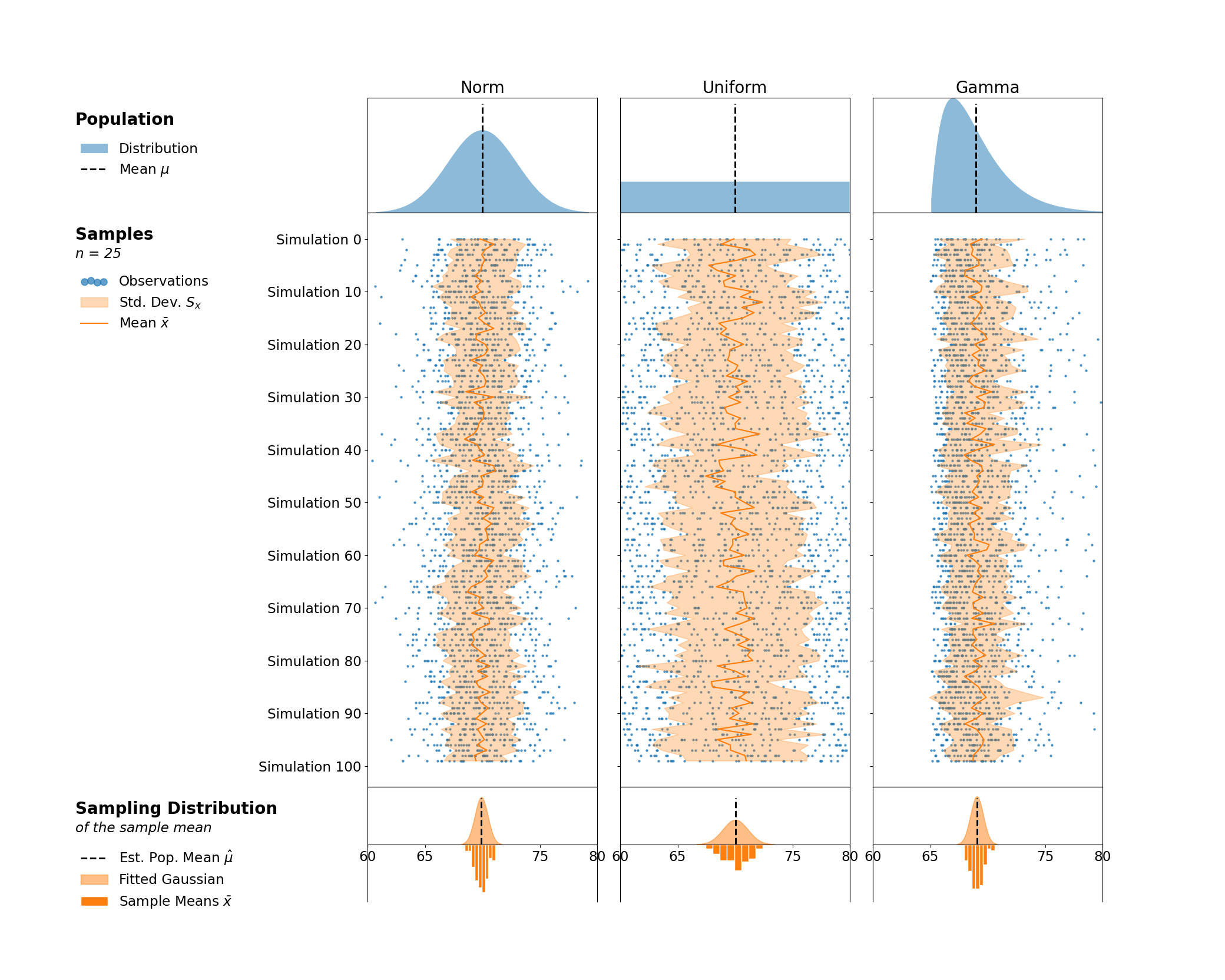
Now, I want to add some horizontal separation to force the viewer to separate the three stages of these plots. I leverage matplotlib's transforms to place a horizontal line that aligns with the bottom of the first and second rows of my Axes and spans the majority of the Figure.
I then use a similar approach to the legend title and subtitle to add a figure title to the top of my Figure. I could have aligned this to my GridSpec instead of on the Figure, but I felt that the center Figure alignment worked better to act as a title for the entire Figure, and not just the 3 columns of plots.
from matplotlib.lines import Line2D

## Add lines to separate rows of plots
for ax in axes[1:, 0]:
    transform = blended_transform_factory(fig.transFigure, ax.transAxes)
    fig.add_artist(
        Line2D([.05, .95], [1, 1], color='lightgray', transform=transform)
    )

for ax in axes[:, 1:].flat:
    ax.yaxis.set_tick_params(left=False)

## Figure title - VPacker with TextAreas enables great control
# over alignment & different fonts
figure_title = VPacker(
    align='center', pad=0, sep=5,
    children=[
        TextArea(
            'Visualizing the Central Limit Theorem',
            textprops={'size': 'x-large', 'weight': 'bold'}
        ),
        TextArea(
            'Sampling Distributions of the Sample Mean',
            textprops={'size': 'large', 'style': 'italic'}
        )
    ])

fig.add_artist(
    AnchoredOffsetbox(
        loc='upper center', child=figure_title,
        bbox_to_anchor=(0.5, 1.0), bbox_transform=fig.transFigure,
        frameon=False
    )
)

display(fig)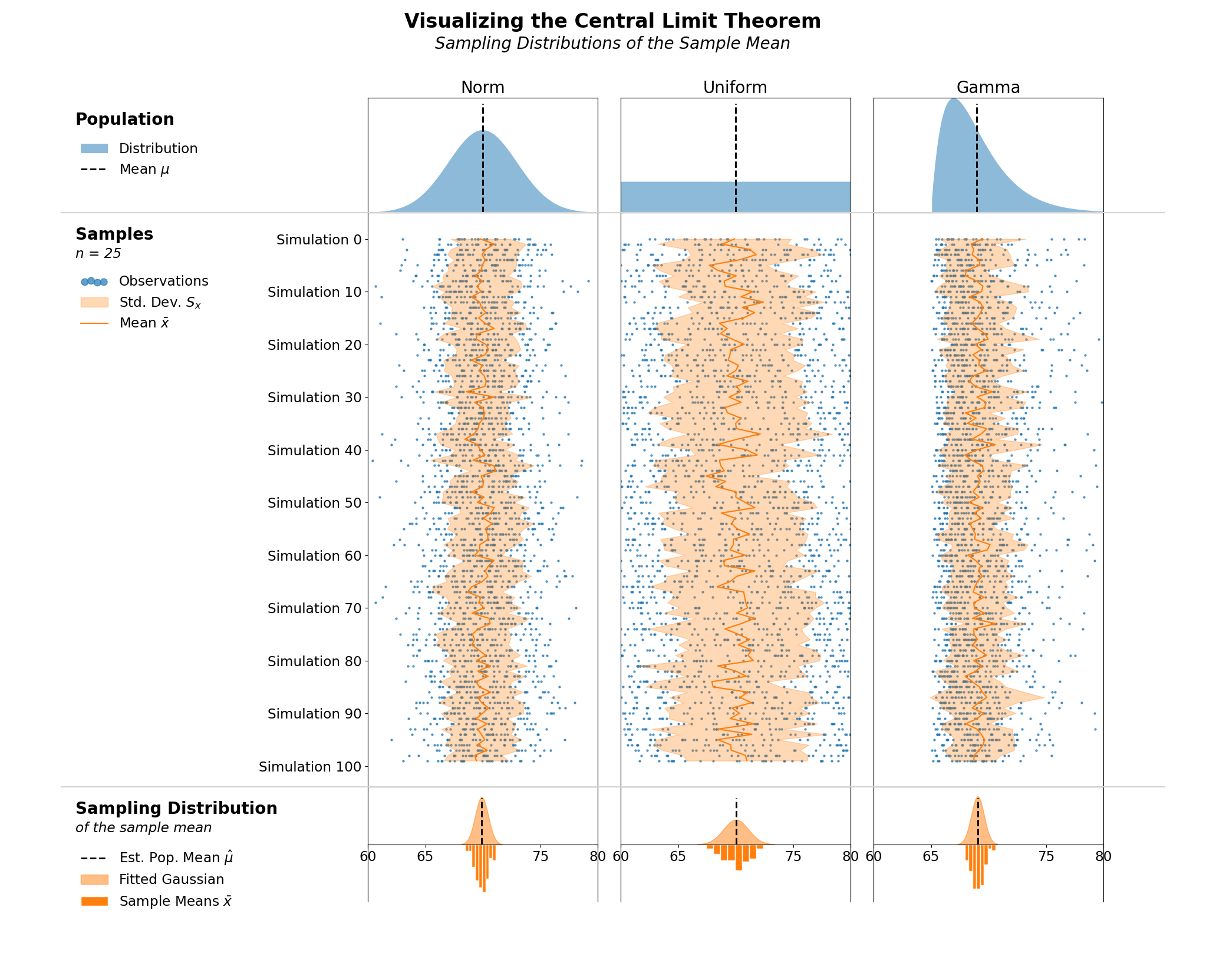
Author Watermark
Finally, I add my company logo as a personal watermark in the lower right corner and remove the Axes.spines from each of the Axes. I am careful to to preserve the bottom spine of my final row of plots since they separate the fitted distribution from the underlying histogram.
from matplotlib.offsetbox import AnchoredOffsetbox, TextArea, DrawingArea
from matplotlib.image import BboxImage
from matplotlib.pyplot import imread

# scaled original dimensions of image to maintain aspect
image_data = imread('../_static/images/DUTC_Logo_Horizontal_1001x61.png')
scaling = 1/3
h, w, _ = image_data.shape
logo_area = DrawingArea(w * scaling, h * scaling)
logo = BboxImage(logo_area.get_window_extent)
logo.set_data(image_data)
logo_area.add_artist(logo)

author = TextArea(
    s='Cameron Riddell @RiddleMeCam', textprops={'color': 'lightgray'}
)
watermark = VPacker(0, 5, children=[logo_area, author])

fig.add_artist(
    AnchoredOffsetbox(
        child=watermark, loc='lower right',
        bbox_to_anchor=(.98, .02), bbox_transform=fig.transFigure,
        frameon=False
    )
)

# Remove the spines
for ax in fig.axes:
    sides = ['bottom', 'left', 'top', 'right']
    if ax in axes[-1, :]:
        sides.remove('bottom')
    ax.spines[sides].set_visible(False)

display(fig)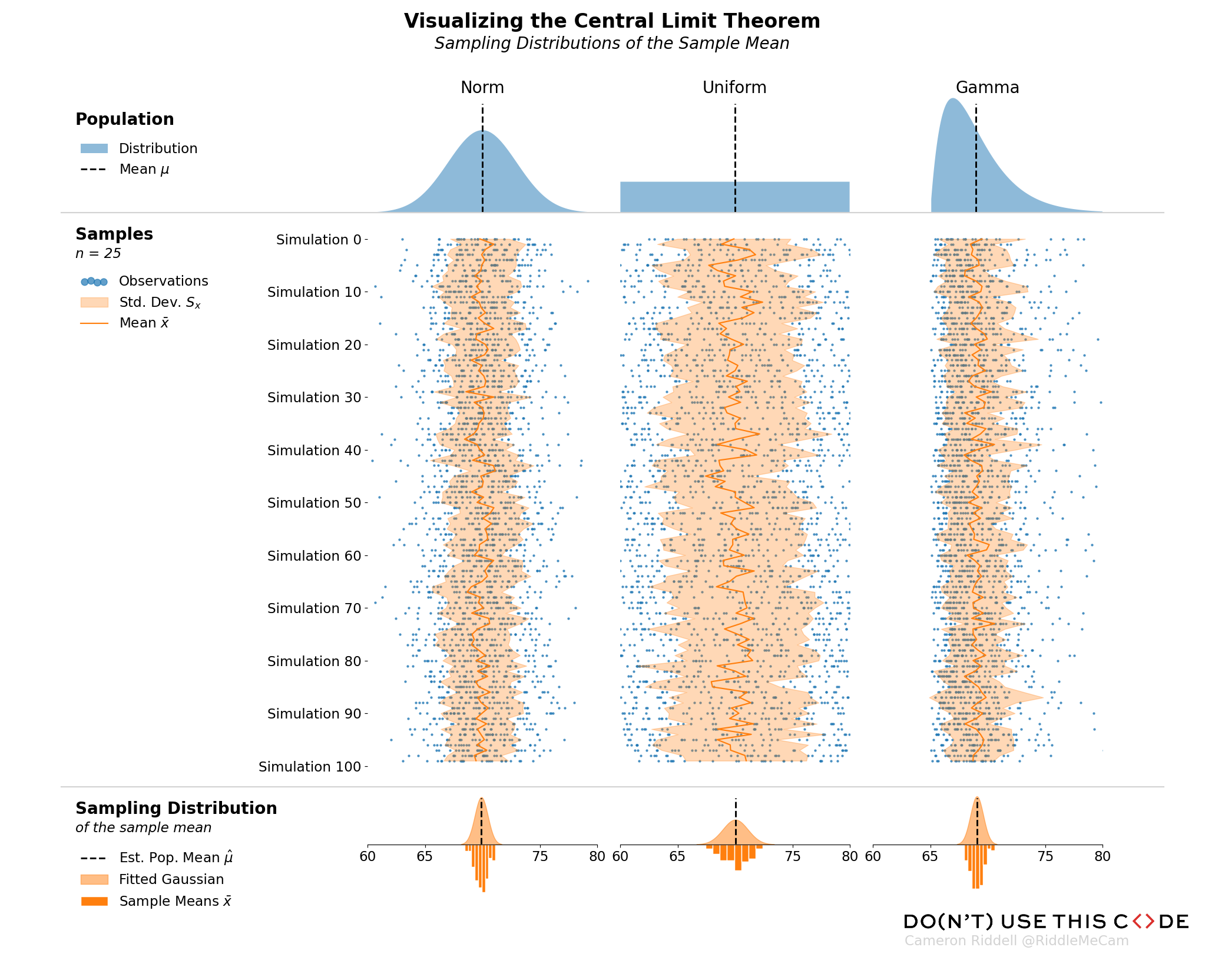
Wrap Up
And that takes us to the end of our Central Limit Theorum visualization. Hopefully you learned a little bit of statistics, as well as some tips you can use to take your matplotlib game to the next level and create refined, communicative data visualizations programmatically. Talk to you all next time!