Statistical Models from formulas
This week, I taught a course on statistical modeling in statsmodels. For those of you who have never used or heard of this Python package, it began as a subpackage in scipy called scipy.models. However, as it grew in size and complexity, it was removed from scipy, and then it became its own package, statsmodels.
As a package, it is a great way to carry out statistical modeling as it provides a great deal of model introspection right out of the box, enabling users to fine-tune their model specification. In this regard, it is similar to the very popular scikit-learn package, but I have found the main difference between the two is that statsmodels is more for introspecting single models, while scikit-learn provides a powerful, object-oriented interface for creating predictive pipelines.
While each of these statistical packages has their place, statsmodels has a home primarily in academic research AND with users transitioning from R to Python.
Patsy: formulaic model specification in Python
The primary reason, statsmodels sees a large influx of R users is due to its explicit support for formula-specified models. The formula mini-language originated in S and was subsequentally implemented in R. The whole idea behind the formula language was to provide a simple interface for representing complex statistical models.
The most common use of fomulas is to allow users to abstract away the construction of design matrices, used very commonly in linear models. While statsmodels does not implement the formula language in Python, it is the only large statistics package that uses them. The actual parsing and construction of the formulas is performed by patsy.
But, before you can really appreciate working with formulas, let's do some linear model fitting (multiple regression) with design matrices we craft by hand.
Creating dummy data
To examine a slightly interesting problem, I wanted to ensure that we had at least two predictive variables to work with: one discrete and one continuous. The continuous values are slightly dependent on the factor creating a slight correlation between them (which we'll ignore).
Importantly, our y values, ys, are highly dependent on predictive variables, which is what we'll try to model.
from pandas import DataFrame
from numpy import array, choose
from numpy.random import default_rng

rng = default_rng(0)
df = DataFrame({
    'factor': rng.choice(['a', 'b', 'c', 'd'], size=100),
}).astype({'factor': 'category'})

df['xs'] = choose(
    df['factor'].cat.codes,
    rng.normal(
        [[60], [50], [40], [35]], scale=5, size=(df['factor'].nunique(), len(df))
    )
)

df['ys'] = (
    df['xs'] - array([50, 40, 30, 20]).take(df['factor'].cat.codes)
    + 20 + rng.normal(0, scale=3, size=len(df))
)

df.head()| factor | xs | ys | |
|---|---|---|---|
| 0 | d | 27.354536 | 28.259441 |
| 1 | c | 39.805825 | 31.084139 |
| 2 | c | 45.331623 | 37.864355 |
| 3 | b | 47.446888 | 27.142061 |
| 4 | b | 49.942335 | 28.892937 |
from matplotlib.pyplot import subplots

fig, ax = subplots()
for factor, group in df.groupby('factor', observed=False):
    p = ax.scatter('xs', 'ys', label=factor, data=group, ec='white')

ax.legend(loc='upper left', bbox_to_anchor=(1, .9), title='factor')
ax.set(xlabel='xs', ylabel='ys')
fig.tight_layout()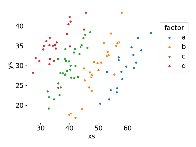
Design Matrices in NumPy
Let's first take the simple route: predict ys directly from xs without worrying about factor.
from numpy.linalg import lstsq
from numpy import column_stack, ones_like
from pandas import get_dummies

# create our design matrix. `xs` is passed through as is
# ones_like represents the intercept of our model
design = column_stack([df['xs'], ones_like(df['xs'])])
design[:5]
array([[27.35453563, 1. ],
[39.80582481, 1. ],
[45.33162277, 1. ],
[47.44688766, 1. ],
[49.94233469, 1. ]])coefs, *_ = lstsq(design, df['ys'], rcond=None)
pred_df = df.assign(pred_ys=design @ coefs)
pred_df.head()
fig, ax = subplots()
ax.scatter('xs', 'ys', data=pred_df, alpha=.8)
ax.plot('xs', 'pred_ys', data=pred_df.sort_values('xs'))[<matplotlib.lines.Line2D at 0x73bae2bb8440>]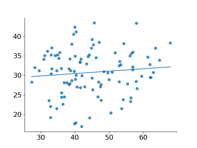
As you can see in the code above, the actual setup of our design was fairly simple—no preprocessing needed to be done, and all we had to do was add a column of 1s to represent our intercept in our least squares operation.
But, what about when we add in a discrete variable such as our factor column? For these values to be appropriately modeled in our design matrix, we will need to sparsely encode them. The most common coding of which is referred to as "dummy coding," and, thankfully, pandas has a function for that.
dummies = get_dummies(df['factor'])
dummies.head()| a | b | c | d | |
|---|---|---|---|---|
| 0 | False | False | False | True |
| 1 | False | False | True | False |
| 2 | False | False | True | False |
| 3 | False | True | False | False |
| 4 | False | True | False | False |
This transforms each level in our factor into its own column. We will need to remove one of these columns (because we are including an intercept in our model, we need to ensure that our columns cannot be linear combination of other columns—there is a lot more to this, but I'll save those details for a future post on linear regression) and combine with our xs column to complete our design matrix.
from numpy import nan
from pandas import get_dummies

dummies = get_dummies(df['factor'])

design = column_stack([df['xs'], dummies.drop(columns=['a']), ones_like(df['xs'])])
design[:5]
array([[27.35453563, 0. , 0. , 1. , 1. ],
[39.80582481, 0. , 1. , 0. , 1. ],
[45.33162277, 0. , 1. , 0. , 1. ],
[47.44688766, 1. , 0. , 0. , 1. ],
[49.94233469, 1. , 0. , 0. , 1. ]])coefs, *_ = lstsq(design, df['ys'], rcond=None)
fig, ax = subplots()
for factor, group in df.groupby('factor', observed=False):
p = ax.scatter('xs', 'ys', label=factor, data=group, ec='white')
ax.legend(loc='upper left', bbox_to_anchor=(1, .9), title='factor')
ax.set(xlabel='xs', ylabel='ys')
fig.tight_layout()
pred_df = df.assign(pred_ys=design @ coefs)
# slight matplotlib trick here- using nan to break apart contiguous lines
pred_df = pred_df.sort_values(['factor', 'xs'], ascending=[False, True])
pred_df.loc[~pred_df.duplicated(['factor'], keep='last')] = nan
ax.plot('xs', 'pred_ys', data=pred_df)[<matplotlib.lines.Line2D at 0x73bae2bd3e90>]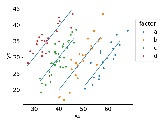
Creating the design matrix by hand isn't too bad, but we lose some at a glance information about what the model is actually comprised of. We would need to be familiar with numpy.column_stack and with pandas.get_dummies in order to make sense of the code above.
This is where patsy and statsmodels come into play.
Linear Regression in Statsmodels
from matplotlib.pyplot import subplots, show
from numpy import column_stack, ones_like, array, choose
from pandas import read_pickle

from statsmodels.formula.api import ols

# model specification: ys predicted by a combination of xs and categorical factors
#   the dummy coding is taken care of for us (Treatment coding by default)
model = ols('ys ~ xs + C(factor)', data=df)
model.exog[:5, :] # design matrix created for us!
array([[ 1. , 0. , 0. , 1. , 27.35453563],
[ 1. , 0. , 1. , 0. , 39.80582481],
[ 1. , 0. , 1. , 0. , 45.33162277],
[ 1. , 1. , 0. , 0. , 47.44688766],
[ 1. , 1. , 0. , 0. , 49.94233469]])fit = model.fit()
# Why not show yet ANOTHER way to plot these data
fig, ax = subplots()
for label, g in df.assign(fitted=fit.fittedvalues).groupby('factor', observed=False):
ax.scatter('xs', 'ys', label=label, data=g, ec='white')
ax.plot(g['xs'], g['fitted'], color='tab:blue')
ax.legend(loc='upper left', bbox_to_anchor=(1, .9), title='factor')
ax.set(xlabel='xs', ylabel='ys')
fig.tight_layout()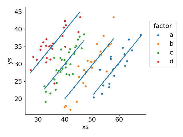
The formula 'ys ~ xs + C(factor)' provides a concise manner of specifying our design matrix, abstracting the need to drop into NumPy ourselves. Furthermore, the ols (ordinary least squares) abstraction enables us to easily model our data and inspect its results. This is a utility that numpy.linalg.lstsq does not provide.
Wrap up
That brings us to a close! This is such a vast topic that I am planning to revisit soon. Hopefully this post left you with some questions about constructing design matrices and how we can use patsy without statsmodels to create them for other programs to use. See you all again next time in a narrower dive into this topic!