Make Your Naive Code Fast with Polars
Welcome back to Cameron's Corner! This week, I presented a seminar on the conceptual comparison between two of the leading DataFrame libraries in the Python Open Source ecosystem: the veteran pandas vs the newest library on the block, Polars.
Polars has been around for over a year now, and since its first release, it has gained a lot of traction. But, what is all of the hype about? Is it some "faster-than-pandas" benchmark? The expression API? Or something else entirely? In my opinion, I'm still going to be using pandas, but Polars does indeed live up to its hype.
The primary difference I observed between the two libraries is this: Due to its expression API, Polars makes it easier to write naive code that works fast.
Polars’ expression API allows it to optimize a query (much like SQL) and efficiently cache intermediates, prune unused logic/projections, and operate in parallel where possible. This means that most of the code you write can be optimized down to more efficient steps that are then executed. On the other hand, this also means the code you write is not necessarily the query that is executed.
For comparison, pandas is very explicit in its nature: what you write is EXACTLY what is executed. This leaves a fairly large gap between fast pandas code and slow pandas code.
A "Fast-Path Pattern" in pandas - Group By
It's no secret that I love pandas and use it almost daily. With this regular use, I have uncovered many approaches to problems that simply work faster than their naive counterparts. The most obvious example of this is understanding how we can work around .groupby(...).apply approaches to distill them into .groupby(...).agg approaches.
For those unfamiliar:
pandas .groupby(...).apply(UDF) operates across the entire dataframe (meaning each entire group of the DataFrame is passed into our user-defined-function)
pandas .groupby(...).agg(NON-UDF) operates on a single column
from numpy import arange
from numpy.random import default_rng
from pandas import DataFrame

rng = default_rng(0)
df = DataFrame({
    'groups': (groups := arange(1000).repeat(100)),
    'weights': rng.uniform(1, 10, size=len(groups)),
    'values': rng.normal(50, 5, size=len(groups))
})

df| groups | weights | values | |
|---|---|---|---|
| 0 | 0 | 6.732655 | 45.775862 |
| 1 | 0 | 3.428080 | 53.759329 |
| 2 | 0 | 1.368762 | 51.352321 |
| 3 | 0 | 1.148749 | 49.757360 |
| 4 | 0 | 8.319432 | 54.192972 |
| ... | ... | ... | ... |
| 99995 | 999 | 3.863986 | 50.054387 |
| 99996 | 999 | 1.494407 | 54.144590 |
| 99997 | 999 | 7.993561 | 34.401766 |
| 99998 | 999 | 6.211353 | 54.042279 |
| 99999 | 999 | 5.556364 | 47.687333 |
100000 rows × 3 columns
The Benchmarks
from dataclasses import dataclass, field
from contextlib import contextmanager
from time import perf_counter

@dataclass
class Timer:
    name: str = None
    start: float = None
    end: float = None

    @property
    def elapsed(self):
        if self.start is None or self.end is None:
            raise ValueError('Timer must have both end and start')
        return self.end - self.start

@dataclass
class TimerManager:
    registry: dict = field(default_factory=dict)

    @contextmanager
    def time(self, name):
        timer =  Timer(name=name, start=perf_counter())
        yield timer
        timer.end = perf_counter()
        self.registry[name] = timer

timer = TimerManager()
While I'm not a huge fan of benchmarks across tools (as I find examples are often cherry-picked for marketing), I think they carry a good amount of meaning when comparing within a specific tool. In this example, we're going to compare a few different approaches when calculating a grouped weighted average in both pandas and polars.
The Naive pandas Approach
This is our first take: the naive approach. This is how someone who is unfamiliar with pandas might approach this problem. We want to calculate a weighted average for each group? Well Pandas has a .groupby(...).apply method that lets us pass each group into a UDF, so we'll go ahead and write a function that operates on 2 Series–one of weights and another of values–and returns an average after multiplying them together. Easy, right?
def weighted_mean(weights, values):
    return (weights * values).sum() / weights.sum()


with timer.time('pandas naive udf') as t:
    df.groupby('groups').apply(
        lambda g: weighted_mean(g['weights'], g['values']),
        include_groups=False
    )

print(f'{t.name} {t.elapsed:.6f}s')
pandas naive udf 0.147143sMaking the most of vectorized operations
Considering the above was a little slow, we might come to realize that our multiplication step is fairly redundant. Why multiply each of these Series per group when we can simply create an intermediate column of the weights * values?
If we sacrifice a little bit of extra memory and then pass a UDF that calculates the mean of these intermediates, we get a HUGE boost in speed!
with timer.time('pandas intermediate UDF') as t:
    (
        df.assign(
            intermediate=lambda d: d['weights'] * d['values']
        )
        .groupby('groups').apply(
            lambda group: group['intermediate'].sum() / group['weights'].sum(),
            include_groups=False
        )
    )

print(f'{t.name} {t.elapsed:.6f}s')
pandas intermediate UDF 0.095506sRemoving All Fastpath Barriers
When it comes to restricted computation domains like pandas, we pay a heavy price for crossing the barrier between Python functions and functions that exist in within that domain. We typically want to push as much of our computation into that domain to best leverage any optimizations or fastpaths that are available.
In the above example, we passed a user-defined function that simply called .mean on each group of the intermediate column we created. pandas cannot "see" into this UDF, and thus cannot leverage any fast paths when performing this operation. If instead we use .groupby(...).mean() or .groupby(...).agg('mean') we can make much better use of pandas internals than we did before to get even better performance.
with timer.time('pandas intermediate fastpath') as t:
    (
        df.assign(
            intermediate=lambda d: d['weights'] * d['values']
        )
        .groupby('groups').agg({'intermediate': 'sum', 'weights': 'sum'})
        .eval('intermediate / weights')
    )

print(f'{t.name} {t.elapsed:.6f}s')
pandas intermediate fastpath 0.010572sPolars Naive Expressions
The thing I enjoy about Polars expression syntax is that they help ensure that the naive approach (like the one we took in the first pandas example) is fast. From a logical understanding, "I want to calculate a weighted mean for each group", it makes sense to use that approach. The expression API helps this method of thinking translate into fast operations.
from polars import from_pandas, col

pl_df = from_pandas(df)

with timer.time('polars naive expression') as t:
    (
        pl_df
        .group_by('groups', maintain_order=True)
        .agg((col('values') * col('weights')).sum() / col('weights').sum())
    )

print(f'{t.name} {t.elapsed:.6f}s')
polars naive expression 0.008849sIf you have been paying close attention- you'll notice that I just recreated my weighted_mean function just using Polars expressions. As it turns out, I did not need to perform this rewrite and instead can use my previous UDF directly provided that it works with expressions. We can verify that it does since calling weighted_mean with column expressions as the input returns a new valid expression:
wmean_expr = weighted_mean(weights=col('weights'), values=col('values'))
wmean_exprWhich means we can use this expression directly in our Polars syntax!
(
    pl_df.group_by('groups', maintain_order=True).agg(wmean_expr)
).head(5)| groups | weights |
|---|---|
| i64 | f64 |
| 0 | 49.681453 |
| 1 | 50.508641 |
| 2 | 50.821316 |
| 3 | 49.808488 |
| 4 | 50.163026 |
We can still create and use UDFs with no performance impact, so long as they take in expressions and output expressions.
Polars is not better because it was written in Rust
Both of these tools have similar performance hits when they encounter opaque barriers. If we use the same .groupby(...).apply(UDF) approach from pandas and have it evaluated by Polars, we see that we lose nearly ALL benefit of the gains that Polars provided to us. Let this be a note that when you're operating within a restricted computation domain, and want your code to run fast, you must play by the rules of that restricted computation domain. In this case, Polars wants you to use its expression API as much as possible, so use it.
from polars import from_pandas, col

with timer.time('polars naive UDF') as t:
    (
        pl_df
        .group_by('groups', maintain_order=True)
        .map_groups(lambda d: weighted_mean(d.select('weights'), d.select('values')))
    )

print(f'{t.name} {t.elapsed:.6f}s')
polars naive UDF 0.297142sPlotting the Benchmarks
It's not a Cameron's Corner without just a little bit of Matplotlib. Here are the benchmarks from each of the approaches we saw above. The Polars expression approach is the fastest, and we can see that no matter what tool we're using, passing in UDFs is going to be slow.
No matter what tool you're using, always think about refactoring away from those user-defined-functions! In some cases, they are impossible to side-step, but in the majority of cases I have seen, they can be worked around.
from flexitext import flexitext
from pandas import Series
from matplotlib.pyplot import subplots, rc
import polars as pl
import pandas as pd
import numpy as np

palette = {'polars': 'tab:blue', 'pandas': 'tab:orange'}

rc('font', size=14)
rc('axes.spines', top=False, right=False)
fig, ax = subplots(figsize=(8, 6), facecolor='white')

s = (
    pd.Series({k: t.elapsed for k, t in timer.registry.items()})
    .sort_values()
)

bc = ax.barh(s.index, s, color=s.index.str.split(' ').str[0].map(palette))
ax.bar_label(bc, [f'{v:.4f}s' for v in s], padding=5)
flexitext(
    x=-.5, y=1,
    s=(
        '<size:x-large>Naive UDF approaches in both'
        f' <color:{palette["polars"]}>Polars <size:medium>{pl.__version__}</></>'
        f' and <color:{palette["pandas"]}>pandas <size:medium>{pd.__version__}</></>'
        ' are SLOW!</>'
    ),
    va='bottom',
)

ax.set_xlabel('Elapsed Time for Operation (s)');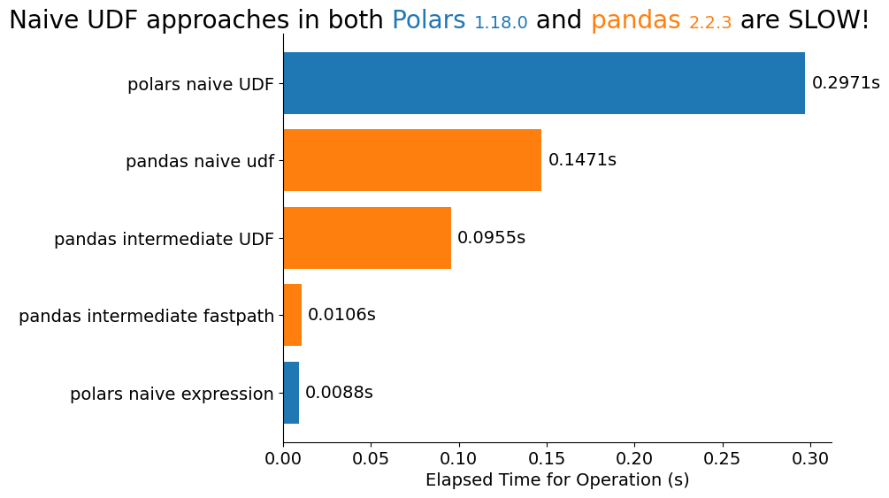
Wrap Up
That's it for this week! Make sure you drop a message on our Discord Server if you enjoyed this blog post. And if you're going to PyCon 2023 this year, make sure you attend James Powell's keynote and say hi! Talk to you all next time!