Useful Multiple-Axis Plots
Welcome back to Cameron’s Corner! This week, in preparation for my upcoming seminar, Intro to Bayesian Stats in Python, we're diving into some (more) data visualization!
I wanted to talk about a question I recently received about Matplotlib, "How do you create a dual-axis chart that conveys unit information?" In my opinion, this is a context where a dual-axis chart is usable and won't mistakenly mislead your audience. Instead of using a second axis to communicate data about a different series of data, we can use a second axis to communicate supplementary information about a single series of data.
The Data
For this week's data viz, we will be revisiting a familiar data set: the amount of fruit I've eaten this past year! This is a fairly straight forward and small set of data. Considering that we are communicating counts of various entities, we may opt to represent this as a bar chart.
Let's take a look at our data and our first viz:
from numpy.random import default_rng
from pandas import Series

rng = default_rng(0)

fruits = ['apple', 'orange', 'banana', 'grape', 'strawberry']
s = (
    Series(rng.integers(20, 100, size=len(fruits)), index=fruits, name='count')
    .sort_values()
)

s
grape 41
strawberry 44
banana 60
orange 70
apple 88
Name: count, dtype: int64Raw Counts OR Percentages?
When we visualize count data, we always have to make a decision:
do we visualize the counts to provide magnitude of each observation to our audience, OR
do we visualize the proportion that each count occupies?
While the relative comparisons in the differing bar heights will be preserved, the raw counts communicate the magnitude of these observations, whereas the use of percentages/proportions communicate a part-of-a-whole relationship.
Let's take a look at both of these visualizations:
from matplotlib.pyplot import rc

rc('figure', facecolor='white', dpi=100)
rc('font', size=16)
rc('axes.spines', top=False, right=False, left=False, bottom=False)
from matplotlib.pyplot import subplots
fig, (ax1, ax2) = subplots(nrows=2)
ax1.barh(s.index, s)
ax1.set_title('I’ve Eaten Apples the MOST over the past year\n(counts)', y=1.03)
ax1.xaxis.grid(visible=True, color='white')
ax2.set_title('(percentages)')
ax2.barh(s.index, s/s.sum())
ax2.xaxis.set_major_formatter(lambda x, pos: f'{x*100:g}%')
ax2.xaxis.set_tick_params(bottom=False)
ax2.xaxis.grid(visible=True, color='white')
fig.tight_layout()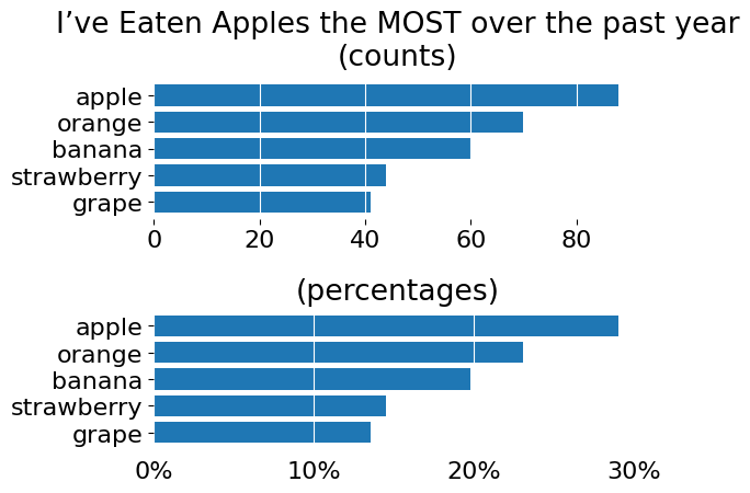
Enhancing the Existing Axis
Instead of visualizing the same data twice, we can create a denser view. One of the most straight forward options will be to add a percentage to the existing raw counts. This can be easily done by changing the major_formatter of the given Axis.
fig, ax = subplots()

ax.barh(s.index, s)
ax.xaxis.set_major_formatter(lambda x, pos: f'{x}\n({100*x/s.sum():.1f}%)')

ax.xaxis.grid(visible=True, color='white')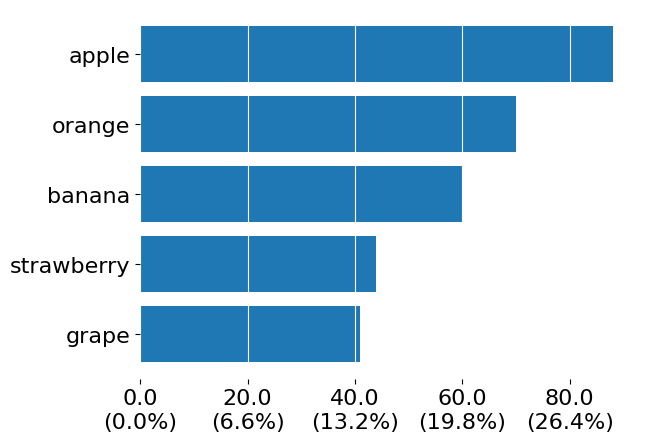
One issue of the above is that, while our percentages are aligned against the counts, this scale increases by 6.6% throughout each tick, which results in odd spacing. Additionally, having the percentages be the same size as the raw counts does not provide any guidance as to which of these values should be the primary thing to look at and which is supplementary.
Separate Axis
Instead of reusing the same axis, we can clone and update it. In this case, we'll clone the full Axes object via twiny() and then scale our visualization from there. We'll create a new tick locator and new tick labels so that the position of the percentage ticks are separate from the raw count ticks. This has the effect of ensuring each Axis has its own sense of scale while accurately represent the underlying data.
from matplotlib.ticker import MultipleLocator

fig, ax = subplots()

ax.barh(s.index, s)

ax2 = ax.twiny()
ax2.set_title('I’ve Eaten Apples the MOST over the past year', pad=5)
ax2.xaxis.set_major_locator(MultipleLocator(s.sum() / 10))
ax2.xaxis.set_major_formatter(lambda x, pos: f'{x/s.sum()*100:g}%')
ax2.xaxis.set_tick_params(labelsize='small')

# Ensure both Axes share the same data space
ax2.update_datalim(ax.dataLim)
ax2.autoscale()
ax2.set_xlim(left=0) # bars charts create 'sticky' edges that begin at 0

ax.xaxis.grid(visible=True, color=ax.get_facecolor())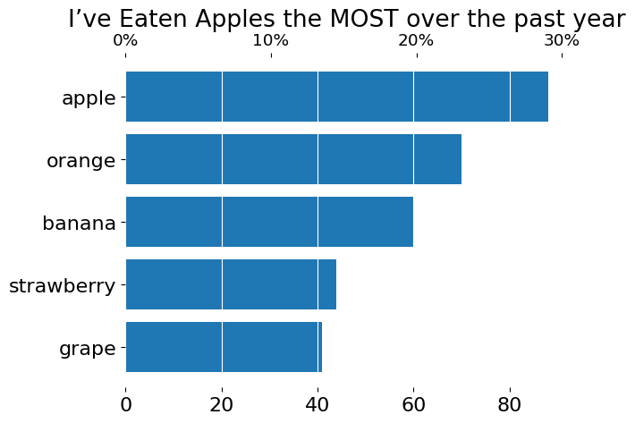
In this instance, I put the percentage ticks on top in a smaller font and the raw counts on the bottom. I could have also put the percentage ticks on the same side of the Axes (e.g., both raw counts and percentages on the bottom) and simply shifted one of those Axis labels so that they do not overlap.
from matplotlib.ticker import MultipleLocator

fig, ax = subplots()

ax.barh(s.index, s)
ax.xaxis.set_tick_params(bottom=False)

ax2 = ax.twiny()
ax2.set_title('I’ve Eaten Apples the MOST over the past year', pad=5)
ax2.xaxis.set_major_locator(MultipleLocator(s.sum() / 10))
ax2.xaxis.set_major_formatter(lambda x, pos: f'{x/s.sum()*100:g}%')
ax2.xaxis.set_tick_params(
    labelbottom=True, top=False, labeltop=False, labelsize='small'
)
ax2.spines['bottom'].set_position(('axes', -.15))

# Ensure both Axes share the same data space
ax2.update_datalim(ax.dataLim)
ax2.autoscale()
ax2.set_xlim(left=0) # bars charts create 'sticky' edges that begin at 0

ax.xaxis.grid(visible=True, color=ax.get_facecolor())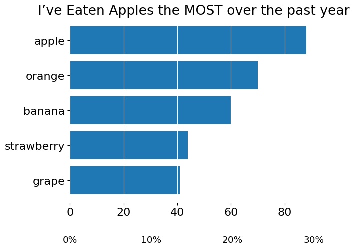
However, I think this approach feels a little clumsy as it's tricky to see the relationship between raw counts and percentages at a glance (which is kinda the main purpose of a graph).
Wrap Up
That’s all we have for this week! Thanks for tuning in and make sure you attend tomorrow's seminar on Bayesian Statistics, as well as next week's seminar on writing your very own Discord bot. See you there!