Timing DataFrame Filters
Hello, everyone! I wanted to follow up on last week's blog post, Profiling pandas Filters, and test how Polars stands up in its simple filtering operations.
An important note: these timings are NOT intended to be exhaustive and should not be used to determine if one tool is "better" than another.
Let's create some dummy data for us to use to investigate:
import pandas; import polars

print(
    f'{pandas.__version__ = }',
    f'{polars.__version__ = }',
    sep='\n',
)
pandas.__version__ = '2.2.3'
polars.__version__ = '1.18.0'from pandas import date_range, DataFrame
from polars import from_pandas, col
from numpy.random import default_rng
rng = default_rng(0)
pd_df = DataFrame({ # ⓐ
'date': date_range(
'2000-01-01', periods=(size:=1_000_000), freq='15s'
),
'value': rng.normal(size=size),
})
pd_df_idx = pd_df.set_index('date') # ⓑ
pl_df = from_pandas(pd_df).set_sorted('date') # ⓒ
pl_lazy = pl_df.lazy() # ⓓ
pl_df.head(5)| date | value |
|---|---|
| datetime[ns] | f64 |
| 2000-01-01 00:00:00 | 0.12573 |
| 2000-01-01 00:00:15 | -0.132105 |
| 2000-01-01 00:00:30 | 0.640423 |
| 2000-01-01 00:00:45 | 0.1049 |
| 2000-01-01 00:01:00 | -0.535669 |
Timing Setup
We will only time each operation once. For the most part, this won't be a huge issue. However, some testing has revealed that pandas is performing some caching, flag setting, or consolidation (unlikely) after its first .loc operation.
This finding warrants further investigation. The objects used to track timings are...
from dataclasses import dataclass, field
from contextlib import contextmanager
from time import perf_counter

@dataclass
class Timer:
    start: float = None
    end: float = None

    @property
    def elapsed(self):
        if self.start is None or self.end is None:
            raise ValueError('Timer must have both end and start')
        return self.end - self.start

@dataclass
class TimerManager:
    registry: list = field(default_factory=list)

    @contextmanager
    def time(self, description):
        timer =  Timer(start=perf_counter())
        yield timer
        timer.end = perf_counter()
        self.registry.append((description, timer))
pandas Filters
For pandas, I wanted to test four approaches:
.loc with a combined boolean mask
.loc using .between (in case any fast paths exist in this approach)
.loc with a sorted index, simply supplying in the start+range of values.
.loc same as the third approach but with a SIGNIFICANT speed difference in the second .loc
from pandas import Timestamp
pd_start = Timestamp(2000, 4, 1)
pd_stop = Timestamp(2000, 4, 2)

timer = TimerManager()

# 1.
with timer.time('pd.loc[start <= date < end]'):
    pd_df.loc[
        (pd_start <= pd_df['date']) & (pd_df['date'] < pd_stop)
    ]

# 2.
with timer.time('pd.loc[date.between(…)]'):
    pd_df.loc[
        pd_df['date'].between(pd_start, pd_stop, inclusive='left')
    ]

# 3.
with timer.time('pd.loc[date] {cold}'):
    pd_df_idx.loc['2000-06-01']

# 4.
# this performs MUCH faster than the above, it is a direct output
# caching because there is still a speed difference even with different inputs
with timer.time('pd.loc[date] {warm}'):
    pd_df_idx.loc['2000-04-01']

for desc, t in timer.registry:
    if desc.startswith('pd'):
        print(f'{desc: >35} → {t.elapsed*1000:.6f}µs')
pd.loc[start <= date < end] → 8.087333µs
pd.loc[date.between(…)] → 6.131260µs
pd.loc[date] {cold} → 77.612707µs
pd.loc[date] {warm} → 1.143518µsPolars Filters
For Polars, I wanted to test some approaches on both an eager polars.DataFrame and a polars.LazyFrame. Aside from the slight differences between the two, the major approaches I wanted to handling the date are...
filter where the start <= date < stop
filter where date.dt.date() == start.date()
slicing, using a binary search for our dates to find slicing indices
from polars import datetime
pl_start = datetime(2000, 4, 1)
pl_stop = datetime(2000, 4, 2)

with timer.time('pl.filter(start <= date < stop)'):
    pl_df.filter(
        (pl_start <= col('date')) & (col('date') < pl_stop)
    )

with timer.time('pl.lazy.filter(start <= date < stop)'):
    pl_lazy.filter(
        (pl_start <= col('date')) & (col('date') < pl_stop)
    ).collect()

with timer.time('pl.filter(date.date == start)'):
    pl_df.filter(
        (col('date').dt.date() == pl_start.dt.date())
    )

with timer.time('pl.lazy.filter(date.date == start)'):
    pl_lazy.filter(
        (col('date').dt.date() == pl_start.dt.date())
    ).collect()

with timer.time('pl[idx_start:idx_stop]'):
    pl_df[
        slice(
            *pl_df.select(
                idx_start=col('date').search_sorted(pl_start),
                idx_stop =col('date').search_sorted(pl_stop)
            ).row(0)
        )
    ]

with timer.time('pl[lazy.idx_start:lazy.idx_stop]'):
    pl_df[
        slice(
            *pl_lazy.select(
                idx_start=col('date').search_sorted(pl_start),
                idx_stop=col('date').search_sorted(pl_stop)
            )
            .collect()
            .row(0)
        )
    ]

for desc, t in timer.registry:
    if desc.startswith('pl'):
        print(f'{desc: >35} → {t.elapsed*1000:.6f}µs')
pl.filter(start <= date < stop) → 7.156336µs
pl.lazy.filter(start <= date < stop) → 10.223621µs
pl.filter(date.date == start) → 10.676583µs
pl.lazy.filter(date.date == start) → 7.588294µs
pl[idx_start:idx_stop] → 5.186307µs
pl[lazy.idx_start:lazy.idx_stop] → 5.903719µsResults
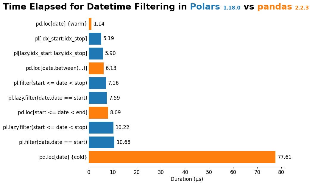
Last—but certainly not least—I wanted to compile all of the timing results and visualize them. Again, these timings are NOT intended to be exhaustive and should not be used to determine if one tools is "better" than another.
df = (
    DataFrame(timer.registry, columns=['description', 'timer'])
    .assign(
        elapsed_us=lambda d: 1_000 * d['timer'].map(lambda t: t.elapsed),
        package=lambda d: d['description'].str.extract('^(pl|pd)'),
    )
    .drop(columns='timer')
    .sort_values('elapsed_us', ascending=False)
)

df| description | elapsed_us | package | |
|---|---|---|---|
| 2 | pd.loc[date] {cold} | 77.612707 | pd |
| 6 | pl.filter(date.date == start) | 10.676583 | pl |
| 5 | pl.lazy.filter(start <= date < stop) | 10.223621 | pl |
| 0 | pd.loc[start <= date < end] | 8.087333 | pd |
| 7 | pl.lazy.filter(date.date == start) | 7.588294 | pl |
| 4 | pl.filter(start <= date < stop) | 7.156336 | pl |
| 1 | pd.loc[date.between(…)] | 6.131260 | pd |
| 9 | pl[lazy.idx_start:lazy.idx_stop] | 5.903719 | pl |
| 8 | pl[idx_start:idx_stop] | 5.186307 | pl |
| 3 | pd.loc[date] {warm} | 1.143518 | pd |
Quite the mix of timings! In this case, it appears that there is not too much of a difference between polars.DataFrame and polars.LazyFrame (these computations aren't incredibly parallelizable, so this is not surprising). We do see a slight increase in the speed of Polars operations that have multiple expressions (see the difference in the Polars Lazy vs eager filter for start <= date <= stop).
Aside from that, the most surprising result is the difference between the cold and warm .loc operations in pandas. This is something I'll explore more in the future, perhaps taking some approaches we saw in Profiling pandas Filters.
%matplotlib inlinefrom matplotlib.pyplot import rc, setp
from flexitext import flexitext
rc('figure', figsize=(10, 6), facecolor='white')
rc('font', size=12)
rc('axes.spines', top=False, right=False, left=False)
palette = {
'pl': '#1F77B4FF',
'pd': '#FF7F0EFF',
}
ax = df.plot.barh(
x='description', y='elapsed_us', legend=False, width=.8,
color=df['package'].map(palette),
)
ax.set_ylabel('')
ax.yaxis.set_tick_params(length=0)
ax.bar_label(ax.containers[0], fmt='{:.2f}', padding=5)
ax.set_xlabel(r'Duration (µs)')
setp(ax.get_yticklabels(), va='center')
ax.figure.tight_layout()
left_x = min(text.get_tightbbox().x0 for text in ax.get_yticklabels())
x,_ = ax.transAxes.inverted().transform([left_x, 0])
annot = flexitext(
s='<size:xx-large,weight:semibold>Time Elapsed for Datetime Filtering in'
f' <color:{palette["pl"]}>Polars <size:medium>{polars.__version__}</></>'
f' vs <color:{palette["pd"]}>pandas <size:medium>{pandas.__version__}</></>'
' </>',
x=x, y=1.02, va='bottom', ha='left',
);
Wrap-Up
What do you think about my approach? Anything you'd do differently? Something not making sense? Let me know on the DUTC Discord server.
That's all for this week! Stay tuned for another dive into DataFrames next week!
Talk to you then!